By Philip Keller, Marketing & Product Management | Metrolab Technology SA
A novel handheld three-axis Hall Magnetometer was introduced at the 2008 Magnetics Conference. In the meantime, this instrument has spawned a family of five, with a range from nanoteslas to 14T, suitable for a wide variety of applications. In this article, we review this family’s technological underpinnings: sensors, electronics, firmware, software and calibration.
 A Family Resemblance: Slender but Powerful
When introduced in 2008, the Three-axis Hall Magnetometer THM1176 surprised by its form factor as well as its functionality. Resembling a mass-market USB device rather than a “gaussmeter”, it simultaneously measures all three components of the magnetic field vector, a feature generally reserved for high-end bench-top systems. This three-axis capability ensures that the vector magnitude B is always known, regardless of the probe’s orientation. An optional palmtop computer provides a completely portable, battery-powered solution.
Since then, additional probes have joined the family, and firmware and software has been perfected, but the basic hardware has remained the same (see Figure 1). The new probes, with their new 3-axis sensors, required developing appropriate calibration techniques. The following sections will examine the underlying technologies.
Magnetometer on a Chip
The sensor of the THM1176-HF (for High Field, see Figure 2) is essentially a magnetometer on a chip (Figure 3). The highest range is sufficient to measure all but the world’s strongest magnets, and the resolution allows accurate measurements of the primary field of conventional magnet systems.
The THM1176-HFC (High Field Compact) uses the same IC, packaged to provide a probe only 0.5 mm thick, well adapted for very small gaps, for example between a stator and rotor. The THM1176-MF (Medium Field) uses a very similar sensor, optimized for higher resolution with smaller ranges: 0.1/0.3/1.0/3.0 T, still amply sufficient for the field strengths encountered in most magnetic systems.

Flux Concentrators and Flux Gates
In contrast, the THM1176-LF (Low Field) uses a conventional arrangement of three individual sensors. Here the emphasis is on maximum sensitivity. A sensor architecture consisting of a microscopic soft-iron flux concentrator and a differential pair of Hall elements increases the sensitivity by approximately a factor of seven, providing µT resolution. The measurement range is limited to 8 mT; at that point the flux concentrator begins to saturate.
Finally, the TFM1186 (Three-axis Fluxgate Magnetometer) uses a recent fluxgate sensor. With its three-axis sensor and low-power operation, this sensor fits right into the THM1176 family, pushing the resolution into the nT range, unachievable with Hall sensors.
Compact, Low-Power and Low-Noise
Whereas the different probes use different sensors, the electronics is common to all probes. In principle, this electronics is very simple, consisting basically of a power supply, digitizer and microprocessor.
In reality, the design is not so simple. The key challenge is to reconcile the conflicting goals of a low-power and low-noise circuit in a minimal footprint. For example, because of the proximity of the components, a switching power supply tended to generate noise in the analog section. The design goals could be met only by exploiting high-density and small-package components destined, for example, for the mobile-phone industry, and by carefully optimizing the analog design.
Full Functionality in Miniature Form
Even in an ultra-compact system, users expect the full functionality provided by a desktop magnetometer: several trigger modes; automatic correction of temperature drift, non-linearity and non-orthogonality; correction of zero offset by the user; range control with optional auto-ranging; controllable measurement averaging; selection of measurement units; and so forth.
In addition, the USB interface implements a palette of widely-used industry standards: USB 2.0, USB Test and Measurement Class (USBTMC), IEEE 488.2, Standard Commands for Programmable Instruments (SCPI), and Device Firmware Update (DFU), along with associated features such as integrated help and status systems.
Modern electronic devices provide ever more functionality in ever-smaller packages by transferring functionality from hardware to firmware (embedded software). The THM1176 family is no different, leveraging to the extent possible the conceptual framework offered by industry standards, the functionality offered by an embedded operating system, specialized functionality offered by third-party packages, and the power of open-source development environments.
Supplying the Missing User Interface
Many instruments come with an installation CD containing a software user interface. For a traditional instrument with a front panel, this is nice to have; for a “black box” peripheral such as the THM1176, it is essential.
Today’s computer platforms allow a much greater sophistication than what is possible on a traditional instrument front panel, and exploiting modern programming languages and frameworks keeps the development effort in check. For example, the THM1176 software includes spectral analysis, which might typically be used to identify power-line noise (50/60 Hz ripple). This powerful feature is in fact easy to implement in the chosen development environment, National Instruments LabVIEW. Also, since the THM1176 complies with the USBTMC and IEEE 488.2 standards, the National Instruments Virtual Instrument Software Architecture (NI-VISA) library provides direct interface support.
Of course, each computer language and development environment also has its pitfalls. LabVIEW is generally known as a “write-only” language, allowing rapid development but rendering code maintenance difficult to impossible. To avoid these pitfalls, an important part of the technology base is a clearly structured design and rigidly consistent implementation.
Getting to Know a Sensor
The last category of essential technological know-how is calibration. At first glance, this appears to be quite trivial, but in fact, developing a calibration procedure is a very humbling experience. Because the different sensors cover a measurement range spanning ten orders of magnitude, no one setup can be used to calibrate all probes. More importantly, this is the moment that previously unsuspected sensor characteristics come to light.
Calibration of the low-field probe, with its soft-iron flux concentrators and differential Hall elements, provides an excellent case study. The measurement range of this probe is below the minimum usually measured by an NMR magnetometer, the “gold standard” for magnetometer calibration. This required developing a completely new calibration setup, based on an AC magnetic field, with a precision fluxmeter acting as reference measurement. To be traceable, the fluxmeter must be calibrated against an NMR magnetometer.
With the calibration setup finally operational, the real fun started. The calibration curve, in addition to the expected nonlinearity, showed a hole in the middle, around B=0. Further experimentation showed that one leg of the curve represented increasing B, and the other decreasing B, for the first time, the hysteresis of the flux concentrator had been made visible. Another puzzling feature were the relatively large angular errors between the three axes. After increasingly desperate attempts to improve the manufacturing process, it became clear that these errors were not due to mechanical positioning, but due to imbalance in the differential pair of Hall elements; the only solution was to calibrate the error and correct for it.
Impressive Today, Awesome Tomorrow
Mastering these diverse areas of technological know-how, sensors, electronics, firmware, software and calibration, represents many man-years of R&D, and has required persistence. Compared to traditional bench-top magnetometers, the resulting product line represents a leap forward: 3-axis measurement; ranges from nT to 14T and from DC to 1 kHz; ultra-compact form factor; full complement of trigger and measurement options; standards-based USB interface; operation with PC/Mac or handheld computer; sophisticated UIF with, for example, spectral analysis and compass display; and, last but not least, traceable calibration.
But as sophisticated as today’s products are, there is still great potential for improvements: even more compact form factor, greater resolution, higher pass-band, improved temperature compensation, interfaces to modern handheld devices… the list goes on. Our idea of a “gaussmeter” is destined to evolve for some time to come.
 About the Author
Philip Keller is responsible for Marketing & Product Management at Metrolab Technology SA, in Geneva, Switzerland, since 2003. His career spans executive management as well as research positions, in a variety of technology industries, ranging from flight simulation to medical ultrasound. He holds Masters degrees in Physics from the Ohio State University and International Management from the University of Lausanne in Switzerland.